A TRANSZMISSZIÓ 1.1  ELMÉLETE
 

Euroconform Regulatory Transmission Modeling for Hungary, Part 1

Dezső J. Szepesi
Katalin E. Fekete
CARM Inc., H-1137 Budapest, Katona J. u. 41. V/25, Hungary

Richárd Büki
MS of HDF, H-1885, P. O. B. 25, Budapest, Hungary, E-mail: rbuki@hotmail.com

Abstract - In Part 1 this paper describes the theoretical and practical steps (correct mathematical and atmospheric-physical simulation, temporal and spatial representativity of input data, scrutinized QA/QC, testing and validation during programming) carried out to achieve a new euroconform regulatory model called TRANSMISSION 1.1 for Hungary.
Simultaneously in another development planetary boundary layer modeling has been prepared including input data standardization and processing for the whole country used by US EPA type AERMOD model family. Description of these efforts will be published in Part 2 in this periodical soon.

Key-words: Actual sector average concentration, centerline concentration, meteorological data base, modeling, most frequent meteorological situations, most probable concentration, norm exceedency, regional scale wind field, regulatory modeling, Szepesi-type stability categories, temporal and spatial representativity of meteorological data, temporal transmission data series, transmission, transmission matrix.

1. Introduction

Recently new euroconform air quality laws ([1], [2], [3] and [4]) were promulgated and adopted for Hungary. To meet the requirements of these laws, the set up of a new regulatory model system named TRANSMISSION 1.1 (in EEA Model Catalogue  HNS-TRASMISSION : .http://pandora.meng.auth.gr/mds/strquery.php?wholedb&MTG_Session=bd2abde34287fec71d8de94715c997fc ) was necessary.

By doing this following principles were honoured:

• Correct mathematical and atmospheric physical simulation,
  
• Scrutinized application of QA/QC procedures during the whole modeling project,
  
• Built-in meteorological database (transmission matrices, time-series, most frequent meteorological situations) for the whole country,
  
• Application of temporally and spatially representative meteorological databases,
  
• Availability of the same standardized transmission model system for users and inspectors ensuring the principle "same input - same output".

2. Concepts and definitions

The first works describing this topic were published in Hungary in 1967, 1970 and 1985.
This article is to present recent developments achieved in this field. We introduce among others a new notion, called average concentration for the actual sector, which is similar to the most probable concentration, but refer to a narrower sector. The difference is in the definition of the borders of the sector. In the new definition we use the concept of Meade and Pasquill [6], this means that the border of the sector is at the line of the 10 per cent value of the ground-level centerline concentration.
It will be shown that this newly introduced notion can be simply estimated by multiplication of the ground-level centerline concentration by a constant. Finally we introduce a new factor which is vital in estimating the norm exceedencies of the 1 hour maximum concentration.
Let us see the basic definition we should use, introducing the concept of the average concentration for the actual sector. The concentration is assumed to have Gaussian distribution.

Figure 1.
The Gaussian distribution and estimation of the different types of concentration

2.1 Estimation of ground-level concentration from an elevated point source

This well-known Gaussian formula specifies the concentration at the ground along the downwind distance of x from a point source:

(1)

Where: X(x,y,0):ground level concentration, µg•m-3
x: the downwind distance from the source, m
y: crosswind distance, m
z: height above the ground, m
E: emission, µg•s-1
pi: constant, 3.1415
sigma y: crosswind dispersion, m
sigma z: vertical dispersion, m
uh: wind speed at source-height, m•s-1
H: effective height of the stack, m.

2.2 Estimation of the ground-level centerline concentration from an elevated point source

This is a special case of Eq. (1) when y=0.

(2)

This type of maximum concentration occurs rarely, but according to the new air quality laws ([1], [2], [3], [4]) this has to be taken into account for determining the range of significant impact for EIA's.

The similar denotations are valid as before.

2.3 Estimation of the most probable concentration

This definition is also introduced by [5]:

(3)

Where:
khi tau: most probable concentration, µg•m-3
y0: crosswind length belonging to meteorological wind sector (22.5o), m
khi centerl: the ground-level centerline concentration, as defined in (2), µg•m-3
The other expressions used are the same, as before.

This type of formula is used in the model for estimation of mean and maximum 24 h and yearly mean ground level concentration.

2.4. Estimation of the average concentration for the actual sector

Based on a suggestion of Meade and Pasquill [6], we define this type of concentration distribution. The concentration is the integral between the 10 percent limits of the ground-level concentration.
In the first step we calculate the limits of the integral, which was in the previous case ±?. Because of symmetry case, y1=y2, the basic equations are:

(4)

Where:
y1, y2: crosswind distances belonging limits of sector delta phi, m

Resulting from this transformation, we have got the average concentration for the actual sector (delta pi). With help of the Taylor-series and the definition of the exponential function:

(5)

Comparing Eq. (3) to the Eq. (5) we can see that the difference between the concentrations calculated between ±? and between the borders suggested by Meade and Pasquill is negligible, only about 2.7%.
Substituting y0 from Eq. (4) and Eq. (5) we have got:

(6)

The multiplication factor 0.57 is a constant, because the crosswind dispersion sigma y effects both khi centerl and y0 similarly, so at the simplification it falls out.
This is the critical formula used by Hungarian environmental inspectors to qualify whether a source complies with norms and the allowable norm exceedencies or not.

3. Practical considerations

The correct estimation of norm exceedencies is vital for air resources management, air quality controll and air quality planning. If we calculate the 1-hour concentration plus the base-pollution, we should divide this sum by a factor denoted by 'e'. So the yearly number of cases,(Nt(w,x)), when concentration is above the limit value is the function of wind direction,w, downwind distance,x, wind speed,u, and atmospheric stability, S, beside of the source parameters:

(7)

Where
- fN1w,u,S : is the number of cases when the sum of the ground-level concentration and basic pollution is over the 1 hour norm with a tolerable degree,
- fN2w,u,S: is the number of cases when the sum of the ground-level concentration and basic pollution exceeds the 1 hour norm more, than tolerable,
- a: the number of cases with allowable exceedencies,
- eN1, eN2: factors of normalization to divide the number of cases fN1w,u,S and fN2w,u,S.

Definition of the factor "e"

Practically the factor "e" is the ratio of the crosswind width of the 22.5o sector and the crosswind width of the sector, where the concentration is greater, than the limit. Starting from this principle, the factor "e" can not be less than 1. As we can see in Fig. 2, the value of "e" varies between 1 and 21 depending on the meteorological and physical conditions.

Figure 2.
The value of "e" at a distance of 2000 m from the source Deduction of algorythm for 'e'

Considering the geometry of Fig. 1 and the definition of the factor "e":

(8)

The inequality, which has to be solved, is:

(9)

After some transformations and defining the ?At as the difference below:

The Eq. (9) has the form:

Where: khi norm: the limit value of the concentration, µg•m-3
At: basic pollution, µg•m-3.

Let us denote a source type factor Q, as:

(10)

We obtain:

Because only the positive resolution of Eq. (8) has physical meaning, so we obtain the following algorithm for the factor "e":

Figure 3.
Yearly number of 1 hour maximum concentration exceedencies around point sources

An example of the yearly number of 1 hour maximum concentration exceedencies estimated by TRANSMISSION 1.0, the official regulatory model in Hungary is shown by Fig. 3 for a two-source configuration with emissions of 400 kg/h and 250 kg•h-1 NO2, stack heights 70 m and 40 m, respectively, and norm of 100 µg•m-3, basic pollution of 20 µg•m-3.

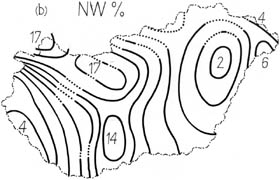
4. Regional scale diffusion climatology

The basic idea of meteorological data preprocessing is that for ground level concentration estimations it is more representative to use regional scale meteorology - in other words average meteorology for an area of 20-30 km diameter - instead of measurements made at a single point. This is called spatial representativity or regionalization of meteorological data. The method of data regionalization is described at [5] here we only summarize the main steps.
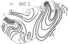
This is a non-computerized (graphical) data assimilation technique. After plotting all wind direction and speed data available (sixteen directions and for each direction mean speed data, respectively) we can analyze these charts graphically, one by one (See Fig. 4 and Fig. 5). Over mountainous areas isofrequencies are denoted by dots. These maps make possible to pick up or interpolate average yearly wind direction frequencies and mean speed values data for any point of the country.

The next step is to preprocess transmission matrices based on 5 years of measurements. This period (1958-1962) was selected because of having similar weather characteristics as the 100-year period (1880-1980) had. In other words the frequency distribution of macrosynoptic (Péczely) weather types were nearly similar in both periods.
The last step is to apply K.Tar's circular polar smoothing process [7] then using interpolation technique built in the model TRANSMISSION 1.1 to interpolate data matrices to any point of interest over the country.
Transmission matrices gained this way and built in the model will be temporally and spatially representative and serve as readily applicable input data base.
Evaluation of the most frequent meteorological situations was another important task. This was carried out by the following way. Since atmospheric stability category S=6 (Szepesi stability 1-7 see [5]) is the most frequent one, surface wind speed prevailing during this stability conditions were evaluated over Hungary. The numerical values ranged from 1.6 m•s-1 to 3.1 m•s-1. These parameters are essentials for the estimation of the range of significant impact (RSI) (1, 2, 3 or 4). Fig.6 shows an example of RSI estimation, for the following source parameters:

Source height 70 m and 40 m, emission 80 kg•h-1 and 50 kg•h-1, u=2,5 m•s-1, basic pollution 20 µg•m-3, norm=100 µg•m-3, surface roughness 0.5 m.

Figure 6.
RSI in km for NO2, emitted by high sources

For estimation of 24 h mean and maximum concentrations time series of meteorological data for 7 regions were included

5. Characteristics of model TRANSMISSION 1.1

By using modules detailed under points 2 and 3 a regulatory model TRANSMISSION 1.0 was prepared to satisfy the new euroconform air quality laws for Hungary.
Major characteristics are the followings: It estimates ground level concentration and deposition emitted by point, area and volume sources - up to 50 -, and located at different points. It calculates 1 h, 24 h and yearly average, maximum values and norm exceedencies. Their outputs are in table or areal distributions on EOV maps in user selected coloured form. Dry deposition and transformation modules are included as well.
Effects of inhomogeneous roughness, basic pollution and orographical effects in homogeneous or inhomogeneous distributions can also be simulated.

6. Summary

Firstly, we reviewed definitions used in the field of air quality modeling, and air quality planning. A new definition, 'the average concentration for the actual sector' was introduced, which is more adequate to the theory of Pasquill and Meade, than the definition used before. It occurs more frequently than the centerline concentration, so it is more realistic for air quality control purposes. Secondly we defined and estimated the normalization factor "e", which is the function of meteorological parameters like wind speed, atmospheric stability, air temperature; and source data like emission of the source, the effective stack height and the distance from the source.

Then we detailed some ideas and steps of carrying out meteorological data preprocessing, the estimation of the range of significant impact and 1 hour maximum concentrations and norm exceedencies by the official, regulatory model TRANSMISSION 1.1 in Hungary.

Literature

[1] Magyar Közlöny (Official Government Gazette) 14/2001. V.9. Emission and Immission Norms. Budapest, Hungary
[2] M.K. ( O.G.G.) 20/2001. II.14. Environmental Impact Assesment. Budapest, Hungary.
[3] M.K., (O.G.G.) 21/2001. II. 14. Clean Air Act. Budapest, Hungary.
[4] M.K., (O.G.G.) 120/2001 VI.30. Modifications. Budapest, Hungary.
[5] Fekete K., Popovics M., Szepesi D., 1983: Légszennyező anyagok transzmissziójának meghatározása ( Guide to Estimate the Transmission of Air Pollutants) OMSZ Hivatalos Kiadványai LV. Kötet
[6] Meade P.J. and Pasquill, F. 1958: A Study of the Average Distribution of Pollution around Staythorpe. Int. Journal of Air Pollution, 1. 60.,
[7] Tar Károly, 1991: Magyarország szélklímájának komplex statisztikai elemzése.(A Complex Statistical Analysis of Wind Climatology in Hungary), OMSZ Kisebb Kiadványai67. szám
[8] Fekete K. and Szepesi D., 1983: Simulation of atmospheric acid deposition on a regional scale. Environmental Management, Vol. 24, pp. 17-28.
[9] Szepesi D., 1967: Légszennyező anyagok turbulens diffúziójának meteorológiai föltételei Magyarországon (Meteorological Conditions of the Turbulent Diffusion of Atmospheric Pollutants in Hungary) OMI Hivatalos Kiadványai XXXII. Kötet
[10] D.J. Szepesi, K.E. Fekete and L.Gyenes: Regularory Models for Environmental Impact Assessment in Hungary. Int. J. Environ. and Pollution, Vol. 5, Nos 4-6, 1995.