IV. Levegőkörnyezeti Szimpózium
1.
Konklúziók
A szimpózium konklúzióit
a Környezetvédelmi és Vízügyi Minisztérium képviseletében Dr. Kovács Endre a következőkben
fogalmazta meg:
A Szimpózium - melynek elsődleges célja a TRANSZMISSZIÓ1.x
hivatalos modell-rendszerhez kapcsolódó témák megvitatása - eredményes
volt.
A Felügyelőségeknél a TRANSZMISSZIÓ1.0 (TR1.0) használata nem
eléggé hatékony, a KHT-k modell
számításokkal történő ellenőrzése kevés. Törekedni kell a TRANSZMISSZIÓS
modell szélesebb körű felhasználására.
Ehhez a szoftver-készítők ismételten felajánlották segítségüket
(lásd 3.1 és 5. pontok).
Fontos a korábbi TR1.0 további finomítása, más szóval kiváltása
a TR1.1 verzióval.
A
szoftverkészítők TR1.1 elnevezéssel az újabb verziót hoztak létre. Az alap
légszennyezettség számítására is alkalmas új modellt (TR1.1) a
Felügyelőségek a LKGSZ Bt. -től 2002 decemberben költségmentesen megkapták.
11 igényes konzultáns cég a TR1.1 modellt adatbázissal
együtt azóta megvette.
Autópályák környezeti hatásvizsgálatánál a légszennyezettség
várható mértéke fontos tényező. Ezért a terjedés meghatározás módszerének
(útmodell) egységesítését jogszabályi környezetben is érvényesíteni kell. A
Minisztérium kér ehhez kapcsolódó
javaslatokat (CALRoads View).
2. Rendezési vonatkozások
Ø Rendezők: Magyar Tudományos Akadémia, Környezetvédelmi és Vízügyi
Minisztérium, Országos Meteorológiai Szolgálat és a Magyar Meteorológiai Társaság.
Ø
Elnök: Rakics Róbert főosztályvezető (Dr. Kovács Endre
főtanácsadó),
Társelnök: Dr. Szepesi Dezső MTA/FTO/MTB
Transzmissziós Rendszer Fejlesztési Albizottság vezetője.
Ø
Téma: A légköri transzmissziós rendszer fejlesztésének
aktuális elvi és gyakorlati kérdései.
Ø
Hely,
idő: Magyar
Tudományos Akadémia Székháza, Felolvasó terem, 2002 szeptember 26, 10-14 h.
Ø
Finanszírozás: A szimpóziumon bemutatott eredményeket 2 éves kutatás-fejlesztés készítette elő,
melynek költségét az OMSZ és a LKGSZ
Bt biztosította.
Ø
Résztvevők:
Ambrózy Pál dr., Antal Emánuel dr., Balogh Beáta,
Bálint Zoltán, Babits Ferenc, Bibók Zsuzsanna, Bunyevácz József, Cz. Péter
(FETIKVF), Daróczi Zsuzsanna, Dubniczky Gyula, Emesz Tibor, Feketéné dr. Nárai Katalin, Gábor
Ildikó, Hangyáné Szalkai Márta, Hajnóczi Miklós, Herczeg Adrienn, Jerszi
László, K.A. (Molnár Kft), K.A. (Promei KHA) Kiss Gabriella, Kovács Endre dr., Koch
Ljudmilla, Koppány György dr.
professzor, Kovács Gábor, Lamatsch Tamás, Lábody Miklós, Lukács
Károly, Major György dr., Marton Sándor dr., Merétei Tamás dr., Mészárosné
Kiss Ágnes, Mika János dr., Mohácsi Ferenc, Nagyné K.L. (Molnár Kft),
Némethné N. Csilla, Paksa Tibor, Pauka Imre dr., Pálfy Miklós Perjés
Katalin, Práger Tamás dr., Pusztainé Holczer Magdolna, Retek Zoltán, Rodé
Lajosné, R.Z. (DDKÖFE), R.ZS. (TENIK), Sámi Lajos, Schauwager Vera, Siedler
Attila, Sivák Szilvia, Steiner Ferenc, Szabó Lászlóné, Szász Józsefné,
Szepesi Dezső dr. Szilágyi Tibor, Tar Károly dr. professzor, Timkó Ildikó,
Tóth László (MSV Rt), Tóth Róbert, Vas Izabella, Vámos Adrienn dr., Zsámbók Zsolt (ADUKVF).
3. Szimpózium előadásainak rövid
összefoglalása
A korábbi - 1995, 99 ill. 2000-ben rendezett
szimpóziumok hozzájárultak ahhoz, hogy a Felügyelőségek és igényes
szakemberek levegőkörnyezeti vizsgálataikhoz már egy év óta hivatalos,
egységes transzmissziós modell rendszerrel és adatbázissal
rendelkezzenek. Röviden szólva: A környezet modellezés ezen a kis
területén megvalósult a következő alapelv: 'azonos inputra - azonos
output'.
Jelen szimpózium feladata,
hogy a számítógépek, adatbázisok, internet adta lehetőségekkel élve elő
kell készíteni a levegőminőség szabályozás döntés előkészítésének korszerű
rendszerét. Ezt úgy célszerű végezni, hogy az egyszerűbb vonatkozásoktól
haladunk a bonyolultabbak felé.
Jelenleg ilyen lépés a modell számítási készség felmérése, mely a
későbbiekben elvezethet a távmodellezésen alapuló döntés előkészítéshez.
Tevékenységünk tudományos
jellegét az biztosítja, hogy a levegőkörnyezeti folyamatok hű szimulálása
mellett, a jól és könnyen működtethető és fokozatosan bővíthető döntés
előkészítő rendszer kialakítására törekszik.
3.1 TRANSZMISSZIÓ1.1 hivatalos
modell rendszer alkalmazása
Előadó: Dr. Szepesi Dezső
A Levegőkörnyezet-gazdálkodási Szaktanácsadó
(LKGSZ) Bt. szakemberei a Felügyelőségek 'levegős' témával foglalkozó
munkatársainak a Szimpózium előtt több héttel egy mintapéldát (2db. NOx
kibocsátó forrás műszaki és környezeti input adatai, ill. a kért output)
küldtek szét. A példa alapján a Felügyelőségeken a TR1.1-val
számításokat végeztek, és a kapott
eredményfájlokat ugyancsak interneten keresztül elküldték. Az eredmények
kiértékelését az alábbi táblázat mutatja.
|
Számítást végző szervezet
|
Számítási eredmények
|
|
Absz. max. konc., mg/m3
|
Órás konc. határé. túllépés évi esete
|
Hatás-terület kiterjedése, km
|
|
Órás
|
Évi
|
|
Környezetvédelmi
Felügyelőség
|
|
|
1.
Észak-Dunántúli
Győr
|
35
|
11,0
|
0
|
1,9
|
|
2.
Közép-Dunavölgyi
Budapest
|
35
|
11,0
|
0
|
1,9
|
|
3.
Alsó-Dunavölgyi
Baja
|
35
|
11,0
|
0
|
1,9
|
|
4.
Közép-Dunántúli
Székesfehérvár
|
35
|
11,0
|
0
|
2,6
|
|
5.
Dél-Dunántúli
Pécs
|
36
|
10,8
|
0
|
2,7
|
|
6.
Nyugat-Dunántúli
Szombathely
|
36
|
10,8
|
0
|
1,9
|
|
7.
Felső-Tiszavidéki
Nyíregyháza
|
35
|
11,0
|
0
|
1,9
|
|
8.
Észak-Magyarországi
Miskolc
|
35
|
11,0
|
0
|
1,9
|
|
9.
Tiszán-túli
Debrecen
|
35
|
11,0
|
0
|
1,9
|
|
10. Közép-Tiszavidéki
Szolnok
|
84*
|
11,2
|
0
|
1,9
|
|
11. Alsó-Tiszavidéki
Szeged
|
36
|
11,0
|
0
|
1,4
|
|
12. Körös-vidéki
Gyula
|
35
|
10,9
|
0
|
1,9
|
|
Főfelügyelőség
Budapest
|
|
|
|
|
|
Szoftver készítő
|
35
|
11,0
|
0
|
1,9
|
* Nem megfelelő összefüggéssel
számított.
A TRANSZMISSZIÓ1.1 Felügyelőségeken való
alkalmazásának további felmérése céljából Dr. Kovács Endre kérdőíves
felmérést végeztetett.
A felmérések alapján megállapítható, hogy a TR1.1
szoftvert a Felügyelőségek szakemberei többnyire jól alkalmazzák. A legtöbb
problémát a hatásterület meghatározása okozta. A hibás értékek itt
általában az NOx (200 mg/m3) helyett az NO2 (100 mg/m3) órás határérték
figyelembe vételéből eredt. Előfordult, hogy az órás maximális koncentráció
számítását az ’aktuális szektorátlagolt’ helyett tévesen a ’szektor
átlagolt’ koncentráció rádió gomb megnyomásával végezték. Indokoltnak
látszik az internetes teszt számítások negyed évente való megismétlése a számítási rutin
karbantartása érdekében. A KHT-k hatósági ellenőrzését megkönnyíti, ill.
gyorsítja (5 perc), ha azok készítői az egységesített ’input lapot’ csatolják (megtalálható: www.levegokornyezet.hu Fogalomkör/ Input adatok).
3.2 Az új TRANSZMISSZIÓ1.1 modell
rendszer bemutatása
Előadó: Feketéné
dr. Nárai Katalin
Saját finanszírozású
kutatások, egy éves tapasztalat, valamint Felügyelőségek javaslatai alapján
az LKGSZ Bt. szakemberei módosították a TRANSZMISSZIÓ1.0 modell rendszert.
Az új verzió a TRANSZMISSZIÓ1.1 elnevezést kapta.
A TR1.1-ben végrehajtott főbb változtatások az
alábbiak voltak: (a) Átalakított összefüggés alkalmazása a 24 órás
koncentráció meghatározására a nagyon ritkán előforduló nem reális 24 órás
koncentrációk kiküszöbölése érdekében, (b) Nyolcnál több forrás (max. 56
forrás) adatbevitelének megkönnyítése, (c) A számítási eredmény ábrájának a
javítása a legkisebb értékű izovonal megjelenítésével, (d) Rajzi opciók
bővítése a háttér objektum behívási lehetőségével, valamint az eredmény
ábrák látványos térbeli megjelenítése (forgatás, döntés, nagyítás, árnyék
hatás stb.).
A Szimpóziumon
egy példa futtatása is megtörtént, amely a TR1.1 használata mellett azt is
bemutatta, hogy a szoftver az alap légszennyezettség modellezéssel való
meghatározására is alkalmas, annak a hatóság által is elfogadott
segédeszköze.
3.3
Alap légszennyezettség méréssel való meghatározása
Előadó: Dr.
Szepesi Dezső; szerzőtársak:
Vámosi Adrienn, Bobvos János, Dubniczky Gyula, Feketéné dr. Nárai Katalin,
Dr. Titkos Ervin
Az alap légszennyezettség hosszúidejű mérési
sorozatból, a mérési adatsorok megfelelő értelmezésével, a helyi hatások
elméleti kiszűrése utján határozható meg.
Az LKGSZ Bt. munkatársai által kidolgozott
módszert az ÁNTSZ szakembereivel közösen Budapest területére alkalmazták. A
mérőállomásokra jellemző lokális hatás meghatározása az állomások bejárása
alapján történt.
Az LKGSZ Bt. szakemberei által kidolgozott
metodika elméleti és gyakorlati vonatkozásai (a Főváros NO2, CO
és SO2 alap légszennyezettségi minta térképei) megtekinthetők a www.levegokornyezet.hu honlapon
(Fogalomköröknél az Alap légszennyezettség és Budapest alap légszennyezettsége címszavaknál
található meg).
3.4 Hatósági útmodellel kapcsolatos problémák
felvetése
Előadók:
Paksa Tibor , Dr. Merétei Tamás ,
Dr. Szepesi Dezső
Az első előadó az autópályákra vonatkozóan a
hatásterület rendeleti meghatározásának szükségességét, ill. az ennél
felmerülő problémákat részletezte.
Egy második előadás hazánkban a gépjármű
közlekedésből eredő emissziókat taglalta számos táblázaton és ábrán
érdeklődésre számot tartó információ bemutatásával.
A fentieken kívül bemutatásra került a gépjármű
közlekedésből eredő légszennyezettség
mértékének meghatározására szolgáló "CALRoads View"
szoftver Demo változata.
3.5 A
levegőkörnyezet klimatikus vonatkozásai
Előadó:
Dr. Koppány György professzor
"Az éghajlat antropogén módosító tényezői és
ezek hatásának természetes korlátai" c. előadás a különböző, egymással sokszor
összhangban nem lévő nézeteket ismertette.
4. Szimpóziumon elhangzott kérdések, válaszok,
ill. hozzászólások
Ø Emesz Tibor
és Dr. Nagy Tibor kollégák felvetették, hogy a TRANSZMISSZIÓ1.0 szoftver Kézikönyvében az elméleti háttéranyagot
is meg kellett volna adni.
Válasz kitért arra, hogy a több, mint 40 oldalas
Kézikönyvet nem lenne szerencsés még további számos oldallal terhelni. Az
elméleti háttéranyag, és egyéb szoftverhez kapcsolódó információ
megtalálható a Levegőkörnyezet-gazdálkodási Szaktanácsadó Bt. honlapján
www.levegokornyezet.hu/Szolgáltatásaink/A Tr1.0 bemutatása alatt.
Ø
Paksa Tibor
szóbeli kiegészítésében hangsúlyozta: Ügyelni kell arra, hogy az órás maximális koncentrációk számítását (mely a hatósági megítélés
egyik fontos paramétere) a TRANSZMISSZIÓ1.1
elfogadása óta az u.n. 'aktuális
szektor átlagolással' kell végezni.
Ø
Emesz
Tibor és kollégái hiányolják, hogy a
TRANSZMISSZIÓ1.1 szoftver a számítási
részeredményeket nem adja meg, noha ezek a hatástanulmányok ellenőrzése
során hasznos ismereteket nyújtanának.
A szoftver készítők bemutatták, hogy a
részeredmények megjelenítése lehetséges. A projektben megadott egy
szennyezőforrásra vonatkozóan megkaphatók, ha az Adat/Teszt feladat adat
menüpontban az input meteorológiát, ill. az outputot kiválasztjuk, majd a
Modell/Teszt feladat menüpontra menve láthatók a kívánt részeredmények.
Ø
Molnár Csilla
és Emesz Tibor a modell
alkalmazásával kapcsolatos
további technikai jellegű kérdéseit
írásban megválaszoltuk.
Ø
Emesz
Tibor kifogásolta, hogy a
TRANSZMISSZIÓ1.1 szoftver a 24 órás
koncentráció számításakor ugyanazt a transzmissziós adatbázist alkalmazza
alacsony és magas forrás esetén is.
A szoftver létrehozók többek között rámutattak, hogy az ország
régióira, reprezentatív évre
óránként előállított transzmissziós adatbázisban az alsó 300 m-es légréteg
stabilitási paramétere szerepel, mely alacsony és magas forrásokra is jó
közelítéssel alkalmazható.
Ø
Mohácsi
Ferenc kolléga hozzászólásában kifejtette, hogy a TR1.1 alkalmazására
szétküldött mintapéldában az órás NOx
határértékként 200 helyett a hibás
100 mg/m3 figyelembe
vétele onnan eredt, hogy többen a
TRANSZMISSZIÓ1.1 szoftver Kézikönyvének 2. kidolgozott példájában lévő NO2
határértéket vették figyelembe.
Ø
Sámi Lajos
írásbeli véleményében megemlíti, hogy az órás maximális koncentrációk az ő modelljétől eltérő eredményeket
adnak.
Ezt
valószínűleg az általa alkalmazott eltérő
algoritmus és adatbázis-beli különbségek okozhatják.
Ø
Emesz Tibor összevetette az ’aktuális szektor
átlagolt’ és a hatásterület meghatározásánál kapott maximális
koncentrációkat.
Ezek eltérésének oka, hogy az érvényes rendelet a
hatásterület meghatározásához a füstfáklya alatti, leggyakoribb
meteorológiai helyzethez tartozó koncentráció alkalmazását írja elő.
5. Modell konzultáció
Szimpózium után a TRANSZMISSZIÓ1.0, ill. 1.1 szoftver készítők konzultációs
lehetőséget biztosítottak. Ezzel a Felügyelőségek szakemberei éltek is.
Számos kérdés merült fel, amely kiterjedt az oldószerek gőzeinek és a
szaghatás szimulálásának lehetőségeire, a számítások részeredményeinek
megismerhetőségére, továbbá az eredmény ábráknak a felhasználó igényeinek
megfelelő átalakítására, stb. A felvetett kérdésekre elsősorban Feketéné
dr. Nárai Katalin részletesen, többnyire számítógépen is illusztrált
formában válaszolt.
A szoftver készítők - a Felügyelőségek szakemberei
által felmerült igény alapján - megígérték, hogy továbbiakban email-en (h11275fek(kukac)ella.hu
vagy szd12506(kukac)ella.hu keresztül segítséget
nyújtanak a szoftver alkalmazásakor felmerülő problémák megoldásában.
A Felügyelőségek
szakemberei időnként (pl. negyedévenként) újabb, egyre nehezebb mintapéldák
szétküldését is hasznosnak tartanák. Amennyiben erre lehetőség nyílik,
a szoftver létrehozók ezt vállalják.
Új hardver kulcsot igényeltek és kaptak a LKGSZ
Bt.-től az ADUKVF és a KOVIKVF
munkatársai.
Dr.
Kovács Endre kifejtette, hogy a
monitor állomások, illetve a 331 mérőhellyel rendelkező félautomatikus
hálózat adatai gyakran nem reprezentatívak, és a mérések adatait hogyan
lehet egy konkrét helyre való vizsgálatnál figyelembe venni. Beszélt a közeljövőben megjelenő, a zónák
besorolását tartalmazó rendeletről, mely több vonatkozásban fog
eligazítást adni.
6. Modell
konzultáció főbb tapasztalatai
Ø
Az órás
maximális koncentráció számításához az ’aktuális szektorátlagolást’ válasszuk.
Ø
Az engedélyezésre benyújtott KHT input adatlappal
egészüljön ki, a számításoknak megfelelő mértékegységekkel.
Ø
A www.levegokornyezet.hu Honlap
Fogalomkörének és Linkjeinek megtekintése számos további kérdésben hasznos
segítséget nyújthat.
Ø
Az új
országos levegő minőségi állomás-hálózat tervezésének szempontjai az EU
adat szolgáltatási igényei mellett a
hazai levegőminőség szabályozás (alap légszennyezettség) elvárásainak biztosításával egészítendők ki. Kulcs fontosságú a
minőség biztosítás és folyamatos minőség ellenőrzés megvalósítása, a korábbi
monitoring programok hibáinak elkerülése érdekében.
Összeállította: Dr. Szepesi Dezső és
Feketéné dr. Nárai Katalin
Jóváhagyta: Dr Kovács Endre
Budapest, 2002. október 20.
AIR QUALITY MANAGEMENT AND
EMISSION INVENTORIES
------
MAJOR REQUIREMENTS
Dezso J. Szepesi
Consultants on
Air Resources Management
Budapest
szd12506@ella.hu,
www.levegokornyezet.hu
Paper presented
at an Expert Meeting Organized by the National Bureau of Statistics on
Integrated Economic-Environmental
Information
Systems at 11-12 November 2002, Budapest Hungary
Ø
Definitions
2. Goals
2.1Territorial
Analysis of Baseline Pollution (Budapest, 2002)
3. Scales, Resolution, Source
Types, and Models for Air Quality Management
4. Rate of Emission (Hungary)
5. Air Quality Levels and
Trends (Hungary)
5.1 Trend
of SO2 (Budapest)
5.2 Most
Severe Smog Situations (Budapest)
5.3
Measured Air and Precipitation Quality Data (Hungary)
6. Retrospective
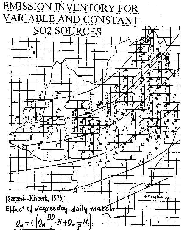
6.1 SO2 Emission Inventory (Pécs, 1975)
6.2 NO2
Emission Inventory for Space Heating
(Budapest, 1985)
6.3 SO2 Emission
Inventory for Space Heating
(Budapest, 1985)
6.4 Air
Quality Control Regions (Budapest,
1985)
6.5
Reginal Scale Emission Inventory EKAR (Hungary, 1989)
7. Conclusions and
Recommendations
a) Definitions
Emission Inventory:
Territorial distribution of pollutant sources (Point, Area and Line) to be
used as model input to estimate or
forecast ground level concentration (isolines).
Two main types exist:
’Bottom-Up’ approach. It is
the end result of rather time consuming data gethering, mostly a field
work. For different source cathegories the rate of emission (e.g. kg/h) is
given by emission factors (kg
emission/goods-production-unit). Emission factors have to be specified by
representative measurements carried
out by Inspectorates. It is more reliable
and gives comparable results. In case of
in advance, systematic, statistical suveying the time demand can be
drastically reduced.
’Top-Down’ approach. It is the result of splitting national or regional fuel
consumption totals according to e.g. inhabitant or
industry ’density’ information. It
is mostly a ’desk work’, giving
rather subjective results.
b) Goals
of Preperation Emission Inventory
To
furnish relevant model input
data for air quality estimations
To use it for territorial analysis of measured
air quality data
c) Scales,
Resolution, Source Types and Models
for Air Quality Management
Scale Effects
Local
0 - 10 Toxic
Urban
10 - 20 Toxic
Regional
20 - 200 Ozone
Continental
200- 2000
Acidifying
Global
> 2000 Green house
gas effect
Scale Source Type Resolution
km2
Local
Point, area, line
-
Urban
Point, area, line 0.5 x
0.5
Regional Area 20 x 20
Continental
Area 50 x
50
150 x 150
Global - -
Scale Goals of modeling Models used
Local
Local impact
TR1.1
Urban
Zoning, AQCR
Roll-back
Urban
Regional
Regional SO2, NO2, Forecast
Ozone
Continental
Abatement LRTP
Forecast
Global Climate modicifation Global
4. Rate of Anthropogenic
Emissions (Hungary, 1985 ), t/yr
Toxic effects
SO2 1.4x10⁶, NOX 2.6x10⁵, TSP 4.5x10⁵,
CO 8.0x10⁵, Pb 6.2x10², Cd 4.4
Ozone precursors
HC 2.3x10⁵, NO2 2.6x10⁵
Acidifying effect
SO2 1.4x10⁶ , NOX 2.6x10⁵, NH3 1.5x10⁵
Greenhouse effects
CO2 8.8x10⁷, CH4 5.3x10⁵, N2O 9.5x10³, Freons 5.5x10³, Halons 6.1x10², TSP
4.5x10⁵
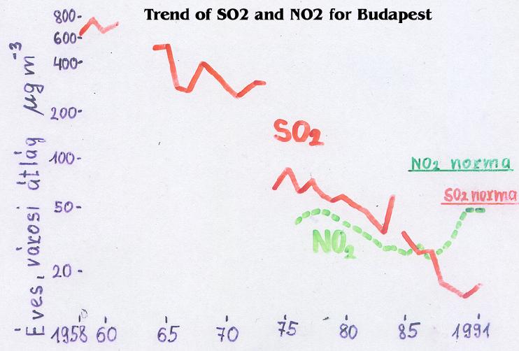
5. Air Quality levels and Trends (Hungary)
Most Severe
Smog Situations (Budapest)
|
Period with Smog
|
Measured
concentrations, µg/m3
|
|
SO2
|
Soot
|
NO2
|
CO2
|
Ózone
|
|
1959March. 16
|
3500-4500
|
5400
|
-
|
-
|
-
|
|
1970Jan. 21-23
|
1500-1800
|
1000
|
-
|
-
|
-
|
|
1989Jan.-Febr.55 days
|
200-670
|
8-350
|
20-200
|
-
|
-
|
|
Smog warning limit values
|
Concentrations µg/m3
|
|
SO2
|
SO2 +
>200ug/m3
Soot
|
NO2
|
CO2
|
Ózone
|
|
Notification
|
400
|
600
|
350
|
20.000
|
180
|
|
Alarm
|
500
|
800
|
450
|
30.000
|
360
|
Measured Air and
Precipitation Quality Data
( Yearly mean, 1985)
Toxic effects
SO2: 13.2 mg m-3, NO2:
7.7 mg
m-3
Pb: 24.8 ng m-3 or
7.8 mg m-3 yr –1
Cd: 0.9 ng m-3 or
0.2 mg m-2 yr-1
Acidifying effects
S: 149 mg H+ m-2 yr–1, N: 112 mg H+ m-2 yr-1
Photooxidants
O3: 120 mg m-3 average max.
200-300 mg m-3 abs.max.
Greenhouse gases
CO2:353-370 ppm, CH4:1,5 ppm, N2O:0.3 ppm,
CFC-11: 280 ppt, CFC-12:
484 ppt
6. Retrospective
7. Conclusions and Recommendations
7.1 To reduce work and shorten time demand
for emission inventories relevant
information on environmental related activities have to be collected in
advance, as part of regular statistical surveying.
7.2 A Base year or Reference year has to be
selected (e.g. 2000) as a starting point for further abatement stategies.
7.3 For abatement strategies, setting up
Zones and AQCR-s (where
necessary) instead of former
’Top-Down’ approach ’Bottom-Up’
method should be used, based on newly prepared census data.
·
For source type categories reliable and domestically
representative emission factors have
to be determined based on emission measurements carried out at
Inspectorates.
·
For Hungary the rate of emission totals can
be characterized as ’low to
medium’. In the late decade it was abated significantly due to
modernization of space heatings and
change in industrial production technology.
·
Air quality levels in Hungary are ’good
to satisfactory’. Traffic
induced pollution in narrow street canyos
with heavy traffic, however, is a real problem and it can be
solved only in the future.
7.7 Severe smog
situations - due to formerly mentioned developments -
are over in Hungary. Major
expenditure for smog relief efforts, are
unnecessary.
7.8 Zones and AQCR-s have already been designed for the
country by using the former
Top-Down approach. A real application
of planned new inventories could be re-design of them. In the era of
micrograms and ppb-s this seems
absolute necessary.
1.4
Summarizing: Emission Inventories
-Are for Urban and Regional
scales models and for analysing measured A.Q. data,
-Worked out by Bottom-Up
approach (based on statistical census data) and checked using regional
totals by Top-Down technique.
-Official Emission
Inventory Guide has to be prepared
forEnvironmental Inspectorates, who are familiar with local and regional
conditions and need E.I.-s as tools in their routine work.
Regulatory
models for environmental impact assessments in Hungary
Int. J. Environment and
Pollution, Vol. 5, Nos. 4-6, 1995
D. J. Szepesi
Air Resources Management Consulting Inc., Katona J.u. 41. V/25
H-1137 Budapest, Hungary
K.E. Fekete and L. Gyenes
Institute for Atmospheric Physics, Hungarian Meteorological Service,
P.O. Box 39, H-1675 Budapest, Hungary
1. Introduction
Based on
ECE Directives1, the requirements of environmental impact assessments
(EIAs) have been regulated in Hungary2,3. On the other hand, the methodology
for atmospheric environmental assessments were standardized (MSZ 21460/1-77
and MSZ 21459/5-85) by the Hungarian Bureau of Standardization in the early
1980s. This methodology has been used to complete more than 150 EIAs. No
complaints have been reported.
This paper describes only the most important charasteristics of models, the
climatological background and some of the results. Further details are
reported in references 4-16.
2. Models
2.1 Model ISAQA
A
Gaussian-plume Industrial Source Air Quality Algorithm (ISAQA) was
developed for the estimation of gaseous pollutant concentrations emitted
continuously from point and area sources and for the deposition of solid
particles during averaging times from 30 minutes to one year4,14. It
considers point and area sources (Figure 4), the plume centreline
concentration for 30 min, sector average values for 24 h and yearly
impacts, transformation, wash-out and deposition of pollutants, HOLLAND or
CONCAWE plume rise, and stack-tip downwash. The model has been validated
for a power plant (1 year) and for a cement plant (6 months). Details are
reported in ref. 9.
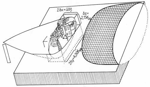
Figure 4.
Consideration of the initial dispersion.
ISAQA
was applied recently to prepare graphical dispersion aid (Figure 5)
for air-quality regulatory authorities to check EIAs prepared by
consultants before giving permits7. The curve in Figure 5 is based on 14.4%
mean highest wind direction frequency and P99%, 30min exceedence.
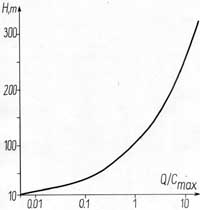
Figure 5.
Dispersion diagram, plotting H (metres) against Q(kg h-1)/Cmax (µg m-3).
2.2 Model URBMOD
URBMOD
can estimate short- and long-term concentrations originating from area
(Gaussian later box) and point (Gaussian) sources in urban areas4,14. It
considers wind direction (29 types of wind pattern), wind speed, mixing
height, initial and regional scale dispersion, pollutant decay, urban
emission inventory and background pollution.
Validation9 was carried out for Pécs, in southern Hungary. The city is
surrounded on the NW to ENE side by mountains. During the 1-year
experiment, the surface wind at ten stations and the upper wind at two
stations were measured four times daily. Orographic temperature gradients
were recorded for stability classification. SO2 concentrations were
estimated over 22 days (Figure 3) by URBMOD, and compared with
values measured at 27 stations in the city. A correlation coefficient of
0.81 was found (Figure 6).
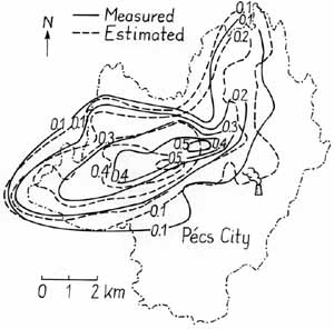
Figure 6.
SO2 concentrations (mg m-3) for Pécs, 29 January 1974.
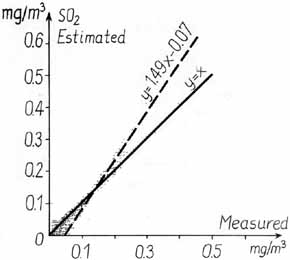
Figure 7.
24 h SO2 concentration scatter diagram for Pécs, 1974; values in mg·
m-3.
2.3 Model
COUNTRYWIDE
The
COUNTRYWIDE model5,6 was designed to estimate seasonal and yearly average
concentrations of gas phase pollutants and the total deposition of
acidifying substances for rural areas, emitted from regional scale domestic
area and elevated sources, as well as from foreign sources. Box and
Gaussian-type algorithms are applied for regional scale emission inventories;
seasonal average wind data of the mixing layer, as well as mixing height
and precipitation data, are considered. Cleansing and deposition mechanisms
are taken into account.
Validation of the model was carried out for the Hungarian Regional Background
Pollution
Stations in different years. Agreement between the measured and estimated
data was satisfactory (relative error <50%).
The model is specially applicable for energy/emission scenario impact
analyses, and to estimate regional scale background pollution for
regulatory use (Figure 8). When such regional background maps are
combined with measured urban concentration patterns (Figure 8a),
differences between regional and urban monitoring can be clearly revealed.
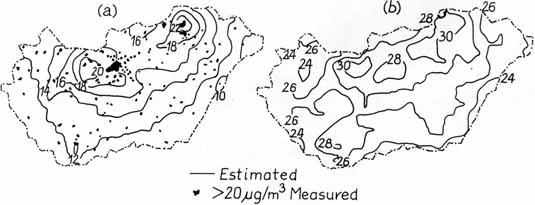
Figure 8 (a) Model estimated and measured yearly SO2
concentrations (µg/m-3) for 1986, and
(b) model estimated yearly total potential acid deposition (10-2 eH+
m-2 yr-1) for 1991 in Hungary.
3. Background pollution
Consistent
estimation of background air pollution originating from larger scale but
less intense polluting sources is of considerable importance for regulatory
applications. Because of he very complex mechanisms involved, a practical
simplifying approach was worked out12,13 (Figure 9). By using this
scheme, contributions from global, continental, regional and urban
background pollution could be easily analysed for any geographic location (Figure
10). Values in Figure 10 mostly represent concentration levels of the
early 1980s. An update would probably furnish values 10-30% lower.
For local regulatory purposes, preparation of regional and urban background
maps for the most important pollutants at 3-year intervals seems
reasonable. The maps should be drawn based on all available measured data
at urban and regional background stations and analysed in the light of
model estimated concentration patterns calculated using the relevant
emission inventory and meteorological input.
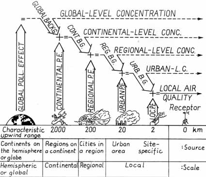
Figure 9.
Hierarchy of air pollution scales (ref. 13)
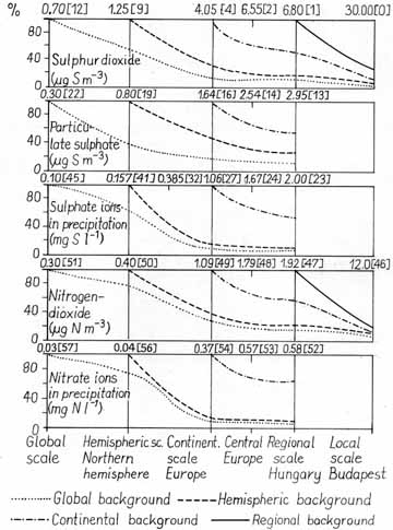
Figure 10.
Contribution from background pollution of sulphur and nitrogen species
4. Transmission matrices
Multidimensional
transmissions matrices are the input bases for long-term estimates of
pollutant concentrations4,10. They were established for 40 stations in Hungary.
For low sources they are based on surface wind direction (16 bins) and
speed (7 bins) records and PGT stability categories using 5 years of SYNOP
data. For medium and high sources, 500 m level wind maps (pilot balloon and
radiosound) were used, together with the stability conditions (7 bins)
estimated on the basis of the lapse rate of the lowest 300 m layer. Between
the 40 points for any location in Hungary, a transmission matrix is
interpolated by using statistics of design wind maps. Applying Péczely-type
Grosswetterlagen (Figure 11/a) analysis15, the period of 1959-1963
was found to best represent the long-term GWL statistics of the base
(1881-1990) interval (Figure 11b).
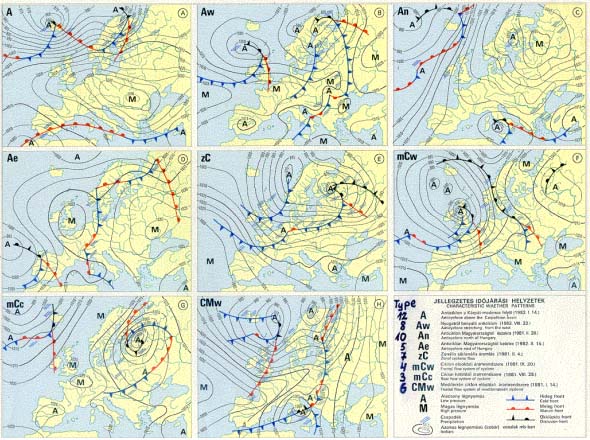
Figure 11/a.
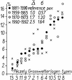
Figure 11/b.
Figure 11a and 11b Relative frequency of 110-year Péczely-type GWL, and
the mean (delta) and standard (sigma) deviations of different short
periods.
5. Design
Winds
The aim
of establishing design wind maps is to furnish readily available regionally
and temporally representative wind statistics for any location in the
country for EIAs. For the analysis of these (Figures 12b and 12c show
sample maps) all available surface wind data series (more than 300 between
1881 and 1980) and upper air ascents (22 long series between 1929 and 1989)
in Hungary were considered16.
Design wind is representative for quasi-level terrain of average roughness
without obstacles. The local effect of extreme roughness, sheltering of
obstacles and mountainous terrain must be model-corrected.
Validation of the design wind concept gave satisfactory results. It also
revealed many inconsistencies in the siting of instruments and former manual
evaluation of wind charts. However, it also confirmed and quantified some
previous findings, for example that the frequencies of the westerlies and
the easterlies over the country are increased by orographic channelling of
the North Carpathian Mountains (Figure 12/a).
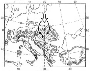
Figure 12/a.
Orograhy of the Central European Region.
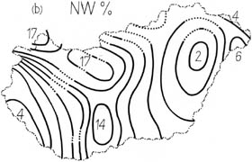 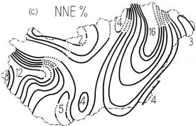
Figure12/b. and 12/c.
Design wind maps: relative frequencies of (b) NW and (c) NNE wind
directions in Hungary.
6.
Stability and dispersion
Atmospheric
stability is estimated in Hungary for low sources by the PGT procedure and
for medium and high sources by the Szepesi method10, based on
classification of temperature lapse-rates of the lowest 300 m layer. The
climatology of the lapse rates is shown in Figure 10. Frequency
distributions were analysed based on six radiosonde ascents daily between
1952 and 1963, resulting in a very characteristic and smooth pattern10.
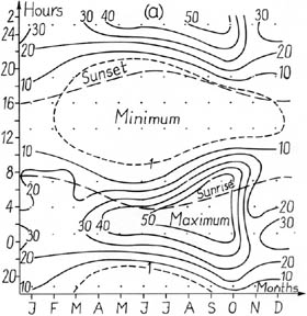 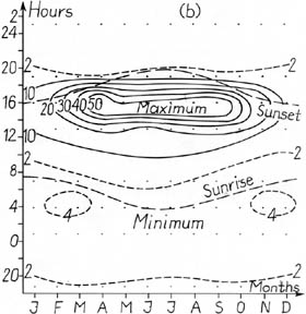
Figure 13.
Relative frequency (%) isopleths of (13a) stable (S=1, 2, 3) and
(13b) superadiabatic (S=7)
stratification of the lowest 300 m layer (1952-1963) at Budapest.
By using
PGT or Szepesi-type stability classes, dispersion coefficients sy and sz
are determined by Nowicki8 formulas:
sigma y=0.08[6p-0.3+1-ln(h/z0)]x0.367(2.5-p)
sigma
z=0.38p1.3[8.7- ln(h/z0)]x1.55exp(-2.35p)
where p
is the exponent of the wind profile equation standardized at 100 m, z0 is
the roughness length, H is the effective height of the effluent, and x is
the distance from the stack.
For deeper air layers, the exponent p and the stability indicators must be
transformed using the diagram shown in Figure 14. This diagram was
constructed using a long series of temperature data measured on high
meteorological towers and by radiosonde11.
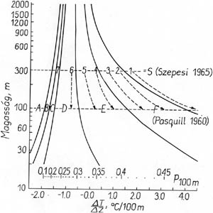
Figure 14
Diagram for the transformation of exponent p and stability indicator S
values.
7.
Conclusions
Regulatory
modellers in Hungary consider that EU initiatives for intercomparison,
harmonization or even standardization are very necessary and important.
Models and input data requirements have been standardized in Hungary.
Preliminary work, however, has been started by the Hungarian Regulatory
Model Improvement Committee (HRMIC) for the preparation of next generation
of models. According to HRMIC, this next generation should include:
- Hybrid
Gaussian models;
- Multidimensional
transmission matrices (similar bins) and data series based on 3 to 10
years of representative SYNOP and radiosonde data; representativity to
be investigated by Grosswetterlagen statistical analysis.
- Design wind
maps and model correction for the effects of obstacles, roughness and
mountainous terrain;
- Dispersion
coefficients based on PBL parameters and radiosonde data with
interpolation possibility using radiation maps;
- Comparisons
and validation exercises.
References
1 ECE
(1987) 'Application of Environmental Impact Assessment', Environmental
Series I.
2 (1993) 'Regulation for Environmental Impact Assessment' (in Hungarian),
86/1993 (VI.4) Korm. rend., Budapest.
3 KTM (1990) 'General content and methodology for environmental impact
assessment of investments' (in Hungarian), Műszaki Irányelv, MI-13-45-1990.
4 Fekete K.E., Popovics M. and Szepesi D.J. (1983) 'Guide to estimate the
transmission of air pollutants', OMSZ Hivatalos Kiadványai, LV, Budapest.
5 Fekete K.E. and Szepesi D.J. (1987) 'Simulation of atmospheric acid
deposition on a regional scale', Environmental Management, Vol. 24,
pp.17-28
6 Fekete K.E. and Gyenes L. (1993) 'Regional scale transport model for
ammonia and ammonium', Atmospheric Environment, Vol. 27A, No. 7, pp.
1099-1104.
7 Fekete K.E.and Szepesi D.J.,. (1994) 'Draft regulation to assess the
stack height for continuously releasing point sources'. KTM, Budapest.
8 Nowicki M. (1976) ' Ein Beitrag zur Bestimmung universeller
Diffusions-koeffizienten', Arch. Met. Geogh. Biokl., Ser. A., No. 25,
pp.31-45.
9 OMSZ (1976) 'Experimental source-receptor relationship investigation in
the region of Pécs' (in Hungarian), Budapest.
10 Szepesi, D.J. (1967) ' Meteorological conditions of the turbulent
diffusion of atmospheric pollutants in Hungary' (in Hungarian), OMI Hiv.
Kiadványai, XXXII, Budapest.
11 Szepesi, D.J. (Editor) (1981) 'Planning of the atmospheric environment'
(in Hungarian), Műszaki Könyvkiadó, Budapest.
12 Szepesi, D.J. (1987) 'Applications of meteorology to atmospheric
pollution problems', WMO Technical Note 188, WMO-672, Geneva.
13 Szepesi, D.J. and Fekete, K.E., (1987) 'Background levels of air and
precipitation quality for Europe', Atmospheric Environment, Vol. 21, No. 7,
pp. 1623-1630.
14 Szepesi, D.J. (1989) 'Compendium of regulatory air quality simulation
models', Akadémia Kiadó, Budapest.
15 Szepesi, D.J. , Szalai, S. and Károssy, Cs. (1993) 'The climatological
characteristics of the atmospheric environment' (in Hungarian), Magyar
Meteorolgóiai Társaság, XXVII, Vándorgyűlés, Debrecen.
16 Szepesi, D.J. and Fekete, K.E., (1993) 'Design wind maps for Hungary'
(in Hungarian), Meteorológiai Tudományos Napok, MTA, Budapest.

MODELL
ÖSSZEHASONLÍTÁS
A TRANSZMISSZIÓ 1.0 (TR1.1) és a korábbi,
kiváltott APOPRO3 (AP3) szoftverekkel, azonos inputokból kiindulva
számításokat végeztünk. A következőkben kis magasságú pontforrásra (amilyen
legtöbbször egy tervezett forrás), illetve egy magas pontforrásra történő
vizsgálat eredményeit mutatjuk be.
A
kiinduló adatok az alábbiak voltak:
h=20 m,
E=1 kg/h, d=0,5 m, v=10 m/s, T=400 K, egyéb tüzelés, felezési idő=100000000
s, x=0,1 km-enként 3 km-ig, zo=0,5 m, határérték=200 mg/m3, alap légsz.=0
mg/m3, u (hatásterületi)=2,5 m/s. Transzmissziós adatbázis: TR1.1 -
Buda7.dat, AP3 - Lorinc.awf.
h=120 m, E=10551 kg/h, d=8 m, v=5,1 m/s, T=434,2 K, egyéb tüzelés, felezési
idő=43200 s, x=0,5 km-enként 20 km-ig, zo=0,5 m. Transzmissziós adatbázis:
TR1.0 - marton6.dat, AP3 - marton.awf.
A távolság függvényében számított rövid-
(órás), illetve hosszú (évi) átlagolású koncentráció maximumok a mellékelt
három ábrán láthatók.
A TR1.1
és az AP3 szoftver alapján végzett fenti, ill. további vizsgálatokból
megállapítható, hogy a TR 1.1-val számított koncentrációk a forráshoz
közelebb kezdenek el nőni, és érik el az AP3-nál többnyire 1,1-2-szer
nagyobb abszolút maximális értéküket. Ezután viszont a TR 1.1-val számított
koncentrációk általában gyorsabban csökkennek.
A
kétféle módszert alkalmazva, 20 m magas forrás esetén a hatásterület
kiterjedését is meghatároztuk. A rendeletben megadottak szerinti
hatásterület meghatározására csak a TR1.0 szoftver képes.
Hatásterület
kiterjedése:
- TR1.0
szerint, a rendeletinek megfelelő módszerrel számított: 0,4 km.
- AP3-ba
beépített, rendeletitől eltérő módszerrel számított: 0,8 ill. 0,9 km.
TR1.0 és AP3 szoftverekkel számított maximális órás koncentráció
20 m magas forrás esetén
TR1.0 és AP3 szoftverekkel számított évi
átlagos koncentráció maximuma
20 m magas forrás esetén
120 m magas forrás esetén
A
TRANSZMISSZIÓ 1.1ELMÉLETE
/To
be published in "Időjárás" soon!/
Euroconform
Regulatory Transmission Modeling for Hungary, Part 1
Dezső J. Szepesi
Katalin E. Fekete
CARM Inc.,
H-1137 Budapest, Katona J. u. 41. V/25, Hungary
Richárd Büki
MS of HDF, H-1885, P. O. B. 25, Budapest, Hungary, E-mail:
rbuki@hotmail.com
Abstract
- In Part 1 this paper describes the theoretical and practical steps
(correct mathematical and atmospheric-physical simulation, temporal and
spatial representativity of input data, scrutinized QA/QC, testing and
validation during programming) carried out to achieve a new euroconform
regulatory model called TRANSMISSION 1.0 for Hungary.
Simultaneously in another development planetary boundary layer modeling has
been prepared including input data standardization and processing for the
whole country used by US EPA type AERMOD model family. Description of these
efforts will be published in Part 2 in this periodical soon.
Key-words:
Actual sector average concentration, centerline concentration,
meteorological data base, modeling, most frequent meteorological
situations, most probable concentration, norm exceedency, regional scale
wind field, regulatory modeling, Szepesi-type stability categories,
temporal and spatial representativity of meteorological data, temporal
transmission data series, transmission, transmission matrix.
1.
Introduction
Recently
new euroconform air quality laws ([1], [2], [3] and [4]) were promulgated
and adopted for Hungary. To meet the requirements of these laws, the set up
of a new regulatory model system named TRANSMISSION 1.1 was necessary.
By doing this following principles were honoured:
- Correct mathematical
and atmospheric physical simulation,
- Scrutinized
application of QA/QC procedures during the whole modeling project,
- Built-in
meteorological database (transmission matrices, time-series, most
frequent meteorological situations) for the whole country,
- Application
of temporally and spatially representative meteorological databases,
- Availability
of the same standardized transmission model system for users and
inspectors ensuring the principle "same input - same
output".
2.
Concepts and definitions
The
first works describing this topic were published in Hungary in 1967, 1970
and 1985.
This article is to present recent developments achieved in this field. We
introduce among others a new notion, called average concentration for the
actual sector, which is similar to the most probable concentration, but
refer to a narrower sector. The difference is in the definition of the
borders of the sector. In the new definition we use the concept of Meade and
Pasquill [6], this means that the border of the sector is at the line of
the 10 per cent value of the ground-level centerline concentration.
It will be shown that this newly introduced notion can be simply estimated
by multiplication of the ground-level centerline concentration by a
constant. Finally we introduce a new factor which is vital in estimating
the norm exceedencies of the 1 hour maximum concentration.
Let us see the basic definition we should use, introducing the concept of
the average concentration for the actual sector. The concentration is
assumed to have Gaussian distribution.
Figure 1.
The Gaussian distribution and estimation of the different types of
concentration
2.1 Estimation of
ground-level concentration from an elevated point source
This
well-known Gaussian formula specifies the concentration at the ground along
the downwind distance of x from a point source:
 (1) (1)
Where:
X(x,y,0):ground level concentration, µg•m-3
x: the downwind distance from the source, m
y: crosswind distance, m
z: height above the ground, m
E: emission, µg•s-1
pi: constant, 3.1415
sigma y: crosswind dispersion, m
sigma z: vertical dispersion, m
uh: wind speed at source-height, m•s-1
H: effective height of the stack, m.
2.2 Estimation of
the ground-level centerline concentration from an elevated point source
This is
a special case of Eq. (1) when y=0.
 (2) (2)
This
type of maximum concentration occurs rarely, but according to the new air
quality laws ([1], [2], [3], [4]) this has to be taken into account for
determining the range of significant impact for EIA's.
The
similar denotations are valid as before.
2.3 Estimation of
the most probable concentration
This
definition is also introduced by [5]:
 (3) (3)
Where:
khi tau: most probable concentration, µg•m-3
y0: crosswind length belonging to meteorological wind sector (22.5o), m
khi centerl: the ground-level centerline concentration, as defined in (2),
µg•m-3
The other expressions used are the same, as before.
This
type of formula is used in the model for estimation of mean and maximum 24
h and yearly mean ground level concentration.
2.4. Estimation of
the average concentration for the actual sector
Based on
a suggestion of Meade and Pasquill [6], we define this type of
concentration distribution. The concentration is the integral between the
10 percent limits of the ground-level concentration.
In the first step we calculate the limits of the integral, which was in the
previous case ±?. Because of symmetry case, y1=y2, the basic equations are:
 (4) (4)
Where:
y1, y2: crosswind distances belonging limits of sector delta phi, m
Resulting
from this transformation, we have got the average concentration for the
actual sector (delta pi). With help of the Taylor-series and the definition
of the exponential function:
 (5) (5)
Comparing
Eq. (3) to the Eq. (5) we can see that the difference between the
concentrations calculated between ±? and between the borders suggested by
Meade and Pasquill is negligible, only about 2.7%.
Substituting y0 from Eq. (4) and Eq. (5) we have got:
 (6) (6)
The
multiplication factor 0.57 is a constant, because the crosswind dispersion
sigma y effects both khi centerl and y0 similarly, so at the simplification
it falls out.
This is the critical formula used by Hungarian environmental inspectors to
qualify whether a source complies with norms and the allowable norm
exceedencies or not.
3. Practical considerations
The
correct estimation of norm exceedencies is vital for air resources
management, air quality controll and air quality planning. If we calculate
the 1-hour concentration plus the base-pollution, we should divide this sum
by a factor denoted by 'e'. So the yearly number of cases,(Nt(w,x)), when
concentration is above the limit value is the function of wind direction,w,
downwind distance,x, wind speed,u, and atmospheric stability, S, beside of
the source parameters:
 (7) (7)
Where
- fN1w,u,S : is the number of cases when the sum of the ground-level
concentration and basic pollution is over the 1 hour norm with a tolerable
degree,
- fN2w,u,S: is the number of cases when the sum of the ground-level
concentration and basic pollution exceeds the 1 hour norm more, than
tolerable,
- a: the number of cases with allowable exceedencies,
- eN1, eN2: factors of normalization to divide the number of cases fN1w,u,S
and fN2w,u,S.
Definition
of the factor "e"
Practically
the factor "e" is the ratio of the crosswind width of the 22.5o
sector and the crosswind width of the sector, where the concentration is
greater, than the limit. Starting from this principle, the factor
"e" can not be less than 1. As we can see in Fig. 2, the value of
"e" varies between 1 and 21 depending on the meteorological and
physical conditions.
Figure 2.
The value of "e" at a distance of 2000 m from the source
Deduction of algorythm for 'e'
Considering
the geometry of Fig. 1 and the definition of the factor "e":
 (8) (8)
The
inequality, which has to be solved, is:
 (9) (9)
After
some transformations and defining the ?At as the difference below:
The Eq.
(9) has the form:
Where:
khi norm: the limit value of the concentration, µg•m-3
At: basic pollution, µg•m-3.
Let us denote a source type factor Q, as:
 (10) (10)
We
obtain:
Because
only the positive resolution of Eq. (8) has physical meaning, so we obtain
the following algorithm for the factor "e":
Figure 3.
Yearly number of 1 hour maximum concentration exceedencies around
point sources
An
example of the yearly number of 1 hour maximum concentration exceedencies
estimated by TRANSMISSION 1.1, the official regulatory model in Hungary is
shown by Fig. 3 for a two-source configuration with emissions of 400 kg/h
and 250 kg•h-1 NO2, stack heights 70 m and 40 m, respectively, and norm of
100 µg•m-3, basic pollution of 20 µg•m-3.
4. Regional scale diffusion climatology
The
basic idea of meteorological data preprocessing is that for ground level
concentration estimations it is more representative to use regional scale
meteorology - in other words average meteorology for an area of 20-30 km
diameter - instead of measurements made at a single point. This is called
spatial representativity or regionalization of meteorological data. The
method of data regionalization is described at [5] here we only summarize
the main steps.
This is a non-computerized (graphical) data assimilation technique. After
plotting all wind direction and speed data available (sixteen directions
and for each direction mean speed data, respectively) we can analyze these
charts graphically, one by one (See Fig. 4 and Fig. 5). Over mountainous
areas isofrequencies are denoted by dots. These maps make possible to pick
up or interpolate average yearly wind direction frequencies and mean speed
values data for any point of the country.
|
Figure 4.
Relative frequencies of NW wind directions
|
Figure 5
Relative frequencies of NNE wind directions
|
The next
step is to preprocess transmission matrices based on 5 years of
measurements. This period (1958-1962) was selected because of having
similar weather characteristics as the 100-year period (1880-1980) had. In
other words the frequency distribution of macrosynoptic (Péczely) weather
types were nearly similar in both periods.
The last step is to apply K.Tar's circular polar smoothing process [7] then
using interpolation technique built in the model TRANSMISSION 1.0 to
interpolate data matrices to any point of interest over the country.
Transmission matrices gained this way and built in the model will be
temporally and spatially representative and serve as readily applicable
input data base.
Evaluation of the most frequent meteorological situations was another
important task. This was carried out by the following way. Since
atmospheric stability category S=6 (Szepesi stability 1-7 see [5]) is the
most frequent one, surface wind speed prevailing during this stability
conditions were evaluated over Hungary. The numerical values ranged from
1.6 m•s-1 to 3.1 m•s-1. These parameters are essentials for the estimation
of the range of significant impact (RSI) (1, 2, 3 or 4). Fig.6 shows an
example of RSI estimation, for the following source parameters:
Source
height 70 m and 40 m, emission 80 kg•h-1 and 50 kg•h-1, u=2,5 m•s-1, basic
pollution 20 µg•m-3, norm=100 µg•m-3, surface roughness 0.5 m.
Figure 6.
RSI in km for NO2, emitted by high sources
For
estimation of 24 h mean and maximum concentrations time series of
meteorological data for 7 regions were included
5.
Characteristics of model TRANSMISSION 1.1
By using
modules detailed under points 2 and 3 a regulatory model TRANSMISSION 1.0
was prepared to satisfy the new euroconform air quality laws for Hungary.
Major characteristics are the followings: It estimates ground level
concentration and deposition emitted by point, area and volume sources - up
to 50 -, and located at different points. It calculates 1 h, 24 h and
yearly average, maximum values and norm exceedencies. Their outputs are in
table or areal distributions on EOV maps in user selected coloured form. Dry
deposition and transformation modules are included as well.
Effects of inhomogeneous roughness, basic pollution and orographical
effects in homogeneous or inhomogeneous distributions can also be
simulated.
6.
Summary
Firstly,
we reviewed definitions used in the field of air quality modeling, and air
quality planning. A new definition, 'the average concentration for the
actual sector' was introduced, which is more adequate to the theory of
Pasquill and Meade, than the definition used before. It occurs more
frequently than the centerline concentration, so it is more realistic for
air quality control purposes. Secondly we defined and estimated the
normalization factor "e", which is the function of meteorological
parameters like wind speed, atmospheric stability, air temperature; and
source data like emission of the source, the effective stack height and the
distance from the source.
Then we
detailed some ideas and steps of carrying out meteorological data
preprocessing, the estimation of the range of significant impact and 1 hour
maximum concentrations and norm exceedencies by the official, regulatory
model TRANSMISSION 1.1 in Hungary.
Literature
[1]
Magyar Közlöny (Official Government Gazette) 14/2001. V.9. Emission and
Immission Norms. Budapest, Hungary
[2] M.K. ( O.G.G.) 20/2001. II.14. Environmental Impact Assesment.
Budapest, Hungary.
[3] M.K., (O.G.G.) 21/2001. II. 14. Clean Air Act. Budapest, Hungary.
[4] M.K., (O.G.G.) 120/2001 VI.30. Modifications. Budapest, Hungary.
[5] Fekete K., Popovics M., Szepesi D., 1983: Légszennyező anyagok
transzmissziójának meghatározása ( Guide to Estimate the Transmission of
Air Pollutants) OMSZ Hivatalos Kiadványai LV. Kötet
[6] Meade P.J. and Pasquill, F. 1958: A Study of the Average Distribution
of Pollution around Staythorpe. Int. Journal of Air Pollution, 1. 60.,
[7] Tar Károly, 1991: Magyarország szélklímájának komplex statisztikai
elemzése.(A Complex Statistical Analysis of Wind Climatology in Hungary),
OMSZ Kisebb Kiadványai67. szám
[8] Fekete K. and Szepesi D., 1983: Simulation of atmospheric acid
deposition on a regional scale. Environmental Management, Vol. 24, pp.
17-28.
[9] Szepesi D., 1967: Légszennyező anyagok turbulens diffúziójának
meteorológiai föltételei Magyarországon (Meteorological Conditions of the
Turbulent Diffusion of Atmospheric Pollutants in Hungary) OMI Hivatalos
Kiadványai XXXII. Kötet
[10] D.J. Szepesi, K.E. Fekete and L.Gyenes: Regularory Models for
Environmental Impact Assessment in Hungary. Int. J. Environ. and Pollution,
Vol. 5, Nos 4-6, 1995.
Proceedings
of the Fourth International Clean Air Congress,
Tokyo, Japan 1978, 284-287
Szepesi D. J.:
Modified
roll-back model for air quality planning
Summary of major findings
For the
quantitative analysis and forecasting of the quality of ambient air proper
tools are necessary. Such tools are meteorological simulation models. In
this paper an advanced version of a simple roll-back model reported by
Moris and Slater (1974) is presented.
This
model is based on the following principle of proportionality: The quality
of air to be attained in the n-th year in an emission control area is
proportional to the air quality measured in the initial year as well as the
quality of air calculated for the n-th year is proportional to the air
quality calculated for the initial year. The above principle of
proportionality is expressed by the following algorythm:
[khi(yn)-khi(b)]goal /
[khi(0ym)-khi(b)]meas. =
sum (i=1...4) {[khi/Q]ni * Q(ni)}calc. /
sum (i=1...4) {[khi/Q]0i * Q(0i)}calc.,
where
khi(yn)
[microgram/cubic m] - the yearly air quality norm value,
khi(b) [microgram/cubic m] - value of background concentration,
khi(0ym) [microgram/cubic m] - yearly mean value of air quality measured
in the emission control area,
index i of the source category is: 1 ground level source, 2 area source,
3 point source, 4 tall stack,
Q(ni) and Q(0i) [t/year] - emission of the i-th source category
in the n-th and the initial year, respectively,
[khi/Q]ni and [khi/Q]0i [microgram/cubic m/t/year] - relative concentration
value of
the i-th source category
in the n-th and the initial year, respectively.
Relative
concentration
|
for
ground level:
|
[khi/Q] (n=0, i=1) = [C1(Z-1.5)M] / [D(uz+0.5)Z x]
|
|
for
area source:
|
[khi/Q] (n=0, i=2) = C2 M / uz T
|
|
for
point source:
|
[khi/Q] (n=0, i=3) = C3 M / [pi e uh sigma(y).sigma(z)
N]
|
|
for
tall stack:
|
[khi/Q] (n=0, i=4) = C4 M / [pi e uh sigma(y).sigma(z)
N]
|
where
C1=7, C2
=30.72 empirical constants,
C3=0.002, C4=0.0006 conversion factors of the one hour maximum concentration
value into yearly average for the whole control area,
M=31700 conversion factor,
Z [m] average height of buildings,
D [m] average width of the main road,
uz, uh [m/s] mean wind speed value at the roof top and at the average
height of the chimneys,
x [m] length of the main roads in the control area,
T [square m] area of the emission control region,
N number of industrial establishments having point sources in the control
area,
sigma(y).sigma(z) [square m] product of the horizontal and vertical
crosswind components of atmospheric dispersion for normal stratification of
the atmosphere, which can be determined by the aid of Figure 1b,
h [m] average height of the chimneys in the emission control area.
Figure 1b.
Product of sigma(y) and sigma(z) against the height of the source
The
model presented gives a good approximation if the following conditions
fulfilled:
a) The
measured air quality data are characteristic for emission control area.
b) The value of background concentration remains unchanged.
c) The diffusion climatological factors will not change during the period
investigated.
The
model presented takes into account the simultaneous polluting effects of
different source categories. According to example shown here, the most
intensive pollution is due to ground level sources as well as area sources.
A much less effect is caused to the ambient air by point sources and tall stacks.
The comparison of the relative concentration values for the 4 source
categories gives the following ratios of the polluting effectiveness:
Ground
level s. : Area s. : Point s. : Tall s. = 500 : 300 : 3 : 1.
References
Morris,
R. et al., Modified Rollback Models. Proc. 5th Expert Meeting on Air
Pollution Modelling. Comitteee on the Challenges to Modern Society, Denmark
(1974).
Journal of Environmental Management (1987) 24,
17-28
Katalin E. Fekete and Dezső J. Szepesi:
Simulation of Atmospheric Acid Deposition
on a Regional Scale
Extended
summary
A
regional scale operational model for the simulation of air and
precipitation quality is presented. The aim of the simulation is to
determine, quantitatively, the complex effects of the following: source
strength of sulphur and nitrogen oxides (Figure 1.), effective height of
the source, wind pattern in the transport layer, mixed layer height,
precipitation, transformation, wet and dry deposition, and hemispheric
background values of air (Table 1.) and precipitation quality.
Figure 1.
Sector zones for which average emission densities were determined
|
Compounds
|
Background, microgram/cubic m
|
|
Sulphur dioxide (in sulphur)
|
1.2
|
|
Particulate sulphate (in sulphur)
|
1.0
|
|
Nitrogen dioxide (in nitrogen)
|
0.4
|
|
Particulate nitrate (in nitrogen)
|
0.05
|
|
Nitric acid gas (in nitrogen)
|
0.05
|
Table 1.
Hemispheric background for sulphur and nitrogen compounds for Europe
The model
presents a regional scale territorial distribution of sulphur dioxide
(Figure 2.), nitrogen dioxide, particulate sulphate and nitrate, nitric
acid gas and precipitation sulphate and nitrate. The total deposition is
also expressed as maximal atmospheric acid stress.
Figure 2.
Annual average sulphur dioxide concentrations (microgram S/cubic m) in
the ambient air originating from domestic area sources (a), domestic tall
stacks (b), and foreign sources (c), 1978-82
The
first-generation model estimates annual average concentrations and
depositions, and it is validated by 5 years of data from Regional
Background Pollution Station in Hungary (Table 2.).
|
|
Compounds
|
Estimated
|
Measured
|
|
Concentration
(microgram/cubic m)
|
Sulphur dioxide (in
sulphur)
|
7.4
|
7.4
|
|
Particulate sulphate
(in sulphur)
|
2.7
|
2.3
|
|
Nitrogen dioxide (in
nitrogen)
|
2.3
|
2.3
|
|
Particulate nitrate(in
nitrogen)
|
0.5
|
0.5
|
|
Nitric acid gas (in
nitrogen)
|
0.5
|
0.6
|
|
Wet deposition
(gram/square m/year)
|
Sulphate (in sulphur)
|
0.93
|
0.95
|
|
Nitrate (in nitrogen)
|
0.36
|
0.28
|
Table 2.
Estimated and measured annual average concentration and deposition values
for the Regional Background Pollution Station at K-puszta (1978-82)
Koncentráció mértékegységek
konvertálása
(Feketéné dr. Nárai Katalain)
Koncentráció mértékegységek
átszámításának általános egyenlete (forrás:
www.air-dispersion.com/formulas.html):
ppmv-ből mg/m3-re
mg/m3 = ppmv *
12.187 * MW /(273.15 + 0C) /1/
Minthogy ppb=10-3 ppmv és mg/m3=10-3
mg/m3, ezért ppb-ből mg/m3-re
való átszámításnál a fenti /1/ egyenlet érvényes, azaz:
mg/m3 = ppb
* 12.187 * MW /(273.15 + 0C) /2/
ahol: MW a szennyezőanyag molekulasúlya
SO2=64,0628 NO2=46,0055 CO=28,0106 O3=47,9982
0C a hőmérséklet,
amelynél az átszámítás történik; általában 20-25 fok.
Legyen 25 0C.
A fenti /2/ egyenlet szerint, a koncentráció
ppb-ből mg/m3-re
való átszámításához az alábbi táblázatban lévő, szennyezőanyagtól függő
szorzótényező (y) alkalmazandó:
|
Szennyezőanyag
típusa
|
y szorzótényező
/mg/m3
= ppb * y/
|
|
Kén-dioxid
|
2,61
|
|
Nitrogén-dioxid
|
1,88
|
|
Szén-monoxid
|
1,14
|
|
Ózon
|
1,96
|
Például 10 ppb kén-dioxid koncentráció esetén 10 * 2,61
=26,1 ~ 26 mg/m3
------------------------------------------------------------------------
|